Analysis of Accuracy Solution and Integral Method for Multi-sound Ultrasonic Flowmeter

Analysis of Accuracy Solution and Integral Method for Multi-sound Ultrasonic Flowmeter

1. Foreword: With the global shortage of energy and water resources, a number of large-scale water conservancy projects and diversion and water diversion projects related to the national economy and people's livelihood have developed rapidly in China, such as the Three Gorges Water Control Project and the South-to-North Water Diversion Project. These projects often include pipes with large calibers and large flows, such as the water inlet pipes of hydropower stations, which cannot be accommodated by conventional flow meters.
The multi-sound ultrasonic flowmeter developed and applied in recent years has better solved the technical problem of large-diameter water flow measurement. The flowmeter manufacturing is not limited by the pipe diameter. The multi-sound path configuration can adapt to the more complicated flow channel structure and flow state. Distribution, so ultrasonic flowmeter has become a good choice for large-caliber water flow measurement [1]. Ultrasonic flowmeter is a speed flowmeter. It calculates the average flow velocity on the acoustic path by measuring the time difference between the downstream and countercurrent propagation of ultrasonic waves in the fluid, and calculates the average flow velocity on the cross section by weighted average by measuring multiple sound path velocities. . Ultrasonic flowmeters require complex calculations to obtain the average flow rate and flow rate of the final flow. The accuracy of the mathematical model used is very important for the overall measurement accuracy.
Obviously, the more the number of sound paths, the higher the accuracy of flow integration, but the increase of the number of sound paths will greatly increase the cost of the flowmeter, so it is very important to choose a reasonable sound path position and matching weight coefficient. Ultrasonic flowmeter can improve the measurement accuracy of the flowmeter itself by improving the measurement accuracy of time and geometric quantity, but the measurement error introduced by numerical integration (referred to as integral error) is always unable to be bypassed by the flowmeter; especially with micro With the rapid development of electronic technology and signal processing technology, the accuracy of sound path speed measurement is getting higher and higher [2-3], and integral error has gradually become a bottleneck for improving the accuracy of flow measurement. For the commonly used 4-channel and 8-channel ultrasonic flowmeters, the integral error is the main source of flowmeter measurement error; for the case of more acoustic paths, the integral error is also an important factor affecting the flowmeter measurement accuracy. Even if the flowmeter installation meets the requirements of the length of the straight pipe before and after, the integral error still exists; and if it cannot be satisfied due to the site or capital limitation, the integral error should be paid more attention.

2, ultrasonic flow meter integration principle:
The ultrasonic flowmeter utilizes the characteristic that the time of propagation of the ultrasonic wave in the fluid is different. The pair of transducers (shown in FIG. 1) placed on both sides of the section to be tested measures the time td, i, of the upstream and countercurrent propagation of the ultrasonic wave. , tu, i, get the average axial velocity of the corresponding sound path [4] (referred to as the sound path speed):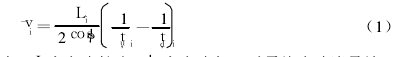



Where: Li is the length of the sound path and i is the sound path angle. For a single-channel flowmeter, the cross-sectional average flow rate has a specific relationship with the acoustic path velocity, but is susceptible to the velocity profile. In order to improve the measurement accuracy of the flowmeter, a plurality of sound paths are arranged in parallel on the section to be tested, and the obtained sound path speed may represent the average speed in the corresponding parallel strips on the section to be measured, as shown in FIG. 2, and The weight coefficient ωi occupied by each strip is calculated by the weighted summation method.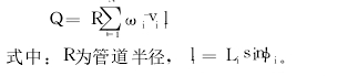




Fig.1 Measurement of sound path velocity (2) Weighted summation method for calculating flow rate Actually, the principle of numerical integration is utilized, and the value of l(z)·v(z) is calculated by a limited number of sound path sampling points to approximate its Definite integral over the interval [ -R, R]: Q = ∫ R - Rl (z) v (z) dz = R ∫ 1-1 l (t R) v (t R) dt ≈ R ∑ Ni = 1 ω il (tiR ) v(tiR)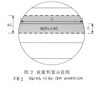


Figure 2 Flow rate calculation diagram: z = t R is the sound path height, t is the relative sound path height, l (z) is the sound path width. Equation (3) transforms the numerical integration into the [ -1, 1] interval to facilitate calculations at different radii. If the sound path width l(z)=2 R2-z2=2R 1 -t2 is substituted, the flow rate is: Q=2R2∫1-1ρ(t)·v(t R)dt≈ 2R2∑Ni=1ωi·v( tiR)· ρ(ti)(4) where: ρ(t) = 1 -t2. Compared with the trapezoidal formula, Simpson's formula and other interpolation type integrals, the sampling point is fixed or even equidistant. The Gauss integral method is a method with high integral precision *** under the limitation of the number of sampling points and the free choice of position. [5]. The ultrasonic flowmeter in the circular tube generally adopts the Gauss-Jaccobi integral method to determine the optimal position ti of the acoustic path and the corresponding weight coefficient ωi, and the number of different sound paths in the IEC41 [6] and PTC18 [7] procedures The acoustic path height and weight coefficient of the time, the ultrasonic probe is generally installed according to the position and coefficient and the flow rate is calculated.

3. Estimation of sound path height and weight coefficient:
3.1, Gauss-Jaccobi program:
According to the Gauss integral theory, the relative acoustic path height ti is the root of the orthogonal polynomial PN(t) with weight ρ(t). For a pipe with a circular cross section, we can see that the weight function is ρ(t) = 1 -t2 from equation (4), which is exactly the weight function of the classical Jaccobi orthogonal polynomial (1 + t) α(1 -t) The special case of β, α = β = κ = 0.5, so the Jaccobi orthogonal polynomial can be recursive by equation (5) [8]: Pj+1 = [ Pj(2j + 2κ+1) x - Pj-1 (j +κ)] (j+κ+1)(j+1)(j+2κ+1)(5) Starting value P-1=0, P0=1. Further, the N roots ti of the PN, that is, the relative sound path height, can be calculated. For rectangular or open channels, the weight function ρ(t)=1 is the Legendre orthogonal polynomial problem. For the circular pipe, the Gauss-Jaccobi solution should be adopted, and the square pipe should adopt the origin of the Gauss-Legendre scheme.
The weight coefficient ωi can be obtained by the following integral: ωi=1ρ(ti)∫1-1ρ(t)∏Nk=0, k≠it-tkti-tkdt (6) combined with the Gamma function Γ(x)=∫∞0e- Ttx-1dt, Equation (6) can be transformed into an easily calculated form: ωi=1ρ(ti)Γ2(κ+N)(κ+N)22κ+1Γ(N+1)Γ(2κ+N+1)PN -1(ti)P'N(ti)(7) where: PN-1(ti) is an N-1 order Jaccobi orthogonal polynomial, and P'N(ti) is a derivative of an Nth order Jaccobi orthogonal polynomial. It is worth noting that the weight coefficient is slightly different from the mathematical Gauss-Jaccobi integral weight coefficient. ρ(ti) is removed from the weight coefficient because the actual sound path width may be different from the installed expected value. Come out, and use the actual measured value ρ(ti)=Lisin i/2 to be substituted in the calculation, as shown in equation (4). Table 1 shows the relative acoustic path height ti and the corresponding weight coefficient ωi for the 4-channel and 9-channel. Since α = β = κ = 0.5 in the Gauss-Jaccobi scheme, a simplified calculation formula for relative acoustic path height and weight coefficient can be obtained mathematically [9]: ti = cosiπN+1, i = 1, 2, ..., Nωi = 1ρ(ti)πN+1sin2iπN+1(8) where: N is the number of sound paths.

3.2, OWICS program:
For the case where the acoustic path velocity distribution v(z) can be expressed by the algebraic polynomial of the corresponding order, the Gauss-Jaccobi scheme has no truncation error; however, there is a big difference between the actual acoustic path velocity distribution and the ideal algebraic polynomial expression, especially It is impossible to reflect the dynamic characteristics of the flow velocity at the pipe wall, which results in a high flow integration result, and the fewer the number of sound paths, the stronger the trend of the flow rate calculation value is higher. Considering that the actual acoustic path velocity distribution of a fully developed circular tube turbulence is close to the exponential distribution of the shape (1 - t2) 1/10, it can be extracted from the acoustic path velocity v(z) to make v'( z) is close to 1, such that v'(z) is more easily expressed as an algebraic polynomial. Further synthesizing it with the weight function ρ(t) =1 -t2: v(z)ρ(t)= v'(z)(1 -t2)1/ 10ρ(t)= v'(z)(1 -t2)0.6= v'(z)ρ'(t) (9) Then according to the new weight function ρ'(t)=(1 -t2)0.6, ie α = β = κ = 0.6, different sounds can be calculated The relative sound path height ti and the weight coefficient ωi of the number of roads N, and the results of the four sound paths and the nine sound paths are shown in Table 1. This algorithm is called the ***ICS section (OWICS) scheme, and is actually a Gauss integration scheme based on orthogonal polynomials [10].

3.3. Comparison of weight coefficient and area average plan:
The Gauss integration scheme has its numerical analysis. Under the determined sound path height, the weight of different sound paths is related to the area of ​​the strip, but it is not proportional. For the calculated relative sound path height ti, the area of ​​the strip where each sound path is located is calculated, and is divided into the middle trapezoid and the bow on both sides for calculation: Si=12(xi+xi+1)Δzi+ΔβiR-sinΔβiR2( 10) where: Δβi= arcsinti-arcsinti+1 is the central angle of the arcuate sides, and xi and xi+1 are the chord lengths of the upper and lower sides of the acoustic strip, which are equally divided between adjacent sound paths The area, the position xi of the string can be solved iteratively using the equal strip area. If the sound path speed is considered to be the average speed in the strip, the area Si of the sound path strip can be used as the weight coefficient when calculating the average speed of the section. In comparison with the previous Gauss integration scheme, the weight coefficient needs to be processed, ωs, i = Si / ρ (ti). Comparing the weight coefficients of the Gauss integration scheme with the area average scheme, it is found that there are differences between the two, as shown in Table 1. Gauss integral scheme is not a simple area-weighted summation. Its weight coefficient is larger than the area weighted average, and the middle sound path is too large and the edge sound path is too small, indicating that the Gauss integral is more emphasis on the intermediate sound path speed versus the average flow rate. The contribution, this may also be the reason why the Gauss integration scheme is more adaptable to the complex sound path velocity distribution than the area average scheme.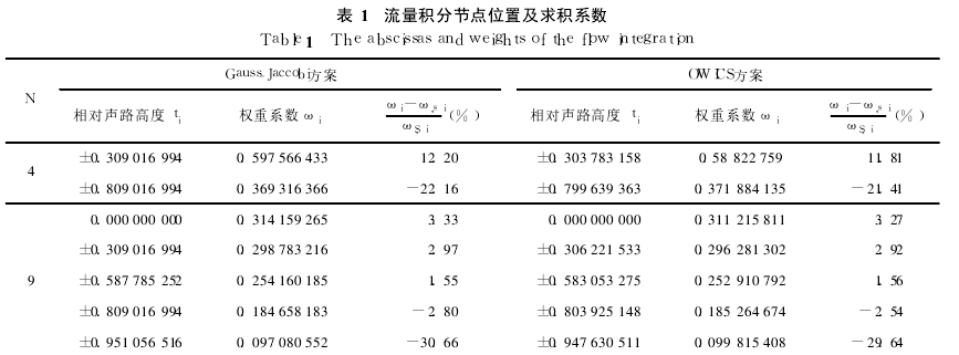



Table 1 Flow integration node position and quadrature coefficient


4. Analysis of flow integral accuracy:
4.1. Integral error when different sound paths are used:
The ultrasonic flowmeter uses a limited acoustic path to restore the velocity profile over the entire section. It is obvious that the more acoustic paths, the more accurate the flow integral. According to the theory of circular pipe turbulence, the fully developed velocity distribution in a circular pipe can usually be described by an exponential distribution. The exponent n is related to the Reynolds number and the relative roughness. Below n=9, v=(1 -r)1 / 9 (0 ≤ r ≤ 1) (11) As an example, the influencing factors of the integral error E=Q-QiQi×100% (12) are analyzed. In the formula, Q is the numerical integration result in different schemes, and Qi is the result of mathematical integration. Figure 3 shows the integration error of the three schemes with different sound paths. It can be seen that the integral error of the Gauss-Jaccobi scheme is greater than zero, and as the number of sound paths N increases, the integral error decreases rapidly. After N=6, the integral error has dropped below 0.05%, and the sound path continues to increase. The number no longer causes a large change, indicating that for simple and smooth flow, too many sound paths have little significance for improving the accuracy of the flowmeter. For the area weighted average scheme, the integral error also decreases as the number of sound paths N increases, but the rate of decrease is very slow, and the integral error of about 0.05% is still maintained at 36 sound paths. A comparison between the two shows that the Gauss integration scheme has higher accuracy than the area-average scheme. For the *** good circular section scheme, the integral error fluctuates around zero, and as the number of sound paths increases, the floating range gradually decreases. For the number of sound paths N = 2 ~ 9, the integral error of the OWICS scheme is slightly smaller than the Gauss-Jaccobi scheme, indicating that the former is indeed better than the latter; but when the number of sound paths is large, the advantage of the OWICS scheme is relatively weak.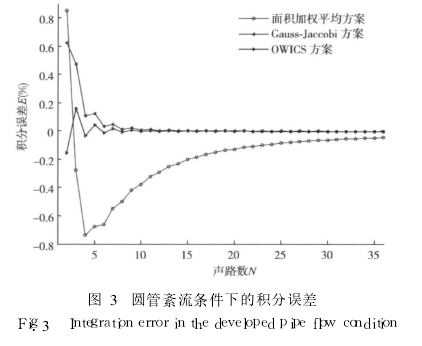



Fig. 3 Integral error under turbulent conditions of a circular tube In order to further explore the difference between the three integration schemes, the classical formula of the turbulent flow field is used:
u(r, θ)=(1 -r)1 /n+mr(1 -r)1/kf(θ) (13) Further analysis of the integral error. Where n, k, m, f(θ) are adjustable parameters, θ is in [ 0, 2π]. Figure 4 shows the calculation results of the integral error of the three schemes. The point value is the mean value of the integral error under a set of flow fields described by equation (13), and the vertical line indicates the standard deviation. The law is similar to the turbulent flow of the tube. The effect of the two Gauss integrals is much better than the area weighted average. The former integral error can not only converge to near zero with the increase of the number of sound paths, but also the amplitude is better than the same sound. The area-weighted average scheme of the number of lanes is small. In addition, the advantages of the OWICS scheme are mainly reflected in the fact that when the number of sound paths is small, if the number of sound paths is limited, it is better to adopt the OWICS scheme.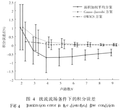


Figure 4 Integral error under spoiler flow field conditions
4.2. Source of integral error:
The Gauss numerical integration process has 2N-1 order algebraic precision, that is, if the actual acoustic path velocity distribution can be expressed by 2N-1 subalgebraic polynomial, the truncation error introduced by the numerical process is zero. However, since the actual sound path velocity distribution curve is affected by boundary conditions and so on, it cannot be expressed by 2N-1 polynomial, so the numerical integration process of flow calculation will introduce a certain truncation error, its size and actual sound path velocity distribution curve. It is related to the fact that the more complex the flow field to be measured, the greater the integral error. The source of the integral error is still explained by taking the exponential flow velocity distribution in equation (11) as an example. The flow rate of this velocity distributed in a pipe with a radius of 1 can be obtained by mathematical integration of Q = 2.678 620. The acoustic path velocity curve in Fig. 5 is obtained by integrating the exponential function. It has a symmetrical distribution characteristic, the middle region is relatively flat, and the vicinity of the edge is rapidly reduced to zero. If the Gauss-Jac-cobi scheme is used to take N = 5 for sampling, the value is The result of the integration is Q = 2.681 950, which is 0.12% different from the true value. Figure 5 also shows the algebraic polynomial family of the set of sampling points (the number of times is not greater than 9, of which 3 gives the constraint of zero boundary), although the curve distribution is more complicated, but the described sound path speed The integral result of the distribution is Q=2.681 950, which is exactly the same as the numerical integration result. This also verifies that the Gauss integral has 2N-1 order algebraic precision. In fact, there is generally no case where the actual acoustic path velocity curve is exactly described by an algebraic polynomial, so there is always an integral error in the integration process.


Figure 5 Schematic diagram of sound path velocity distribution

Gauss-Jaccobi integral method and OWICS integral method are based on the assumption that the sound path velocity distribution can be expressed by algebraic polynomial. Some researchers believe that the sound path velocity distribution is not suitable for expression by algebraic polynomial [12], especially for flow. In the case of disturbance of the field, A.Nichtaw-itz [13] considered that it is appropriate to use the PCHIP polynomial (segmented stereo Hermitian interpolation polynomial) to express the flow velocity distribution. In the case of correcting the side wall flow field, 4 sound paths are used. The PCHIP integration method has approximately the same integral error as the 9-channel Gauss-Jaccobi integration method. In addition, some scholars [14-15] believe that the flow field flow is very complicated and unpredictable, and the use of complex channel arrangement and neural network for processing ideas to promote the mathematical model of ultrasonic flowmeter.


5 Conclusion:
This paper analyzes the flow integral principle of ultrasonic flowmeter, and combines the numerical analysis theory to derive the sound path height and weight coefficient of the ultrasonic flowmeter sound path layout scheme (Gauss-Jaccobi scheme and OWICS scheme). By comparing the weight coefficient difference between the Gauss integral method and the area weighted average method at the same acoustic path height, it is found that the Gauss integral method pays more attention to the contribution of the middle part of the sound path to the average flow velocity, which may be an important reason for its higher accuracy. In addition, the causes of the flow integration error of Gauss integral scheme are analyzed, and the influence of the number of sound paths on the integral error is compared. The integral error is derived from the fact that the actual sound path speed cannot be expressed by algebraic polynomial; the more the number of sound paths, the higher the integral accuracy, but the excessive number of sound paths is not significant for improving the accuracy of the flowmeter.

Clear Flat Bag

Clear Flat bag is made from Food Grade Virgin material. environmentally friendly and hygienic. They are water-proof, Moisture-proof, strong toughness, tear resistance, good for storage and usually for packing sugar, biscuits, candy, coffee bin, fruits , drinks or other foods. Normally width from 3 inch to 12 inch. Length from 7 inch to 22 inch. Material could be in HDPE or LDPE.

Clear Flat Bags, Polyethylene Flat Bags, Clear Flat Polyethylene Bag, Side Seal Bag, Clear Bag, Crystal Clear Side Gussets Bags

BILLION PLASTIC MANUFACTURING CO.,LTD, JIANGMEN , https://www.jmflatbag.com